Liquid Neural Networks - A Modern Approach

Introduction

Liquid neural networks, a relatively new concept, represents a paradigm shift in how we design, train, and deploy computational models inspired by biological systems. Unlike traditional deep neural networks, which generally rely on fixed architectures and static parameters once trained, liquid neural networks—often referred to as liquid time-constant networks—are dynamic, continually adapting their internal parameters in response to changing inputs and conditions. It draws inspiration from how natural biological neurons operate in real neural circuits, where synaptic strengths and temporal patterns of neural firing evolve continuously, enabling brains to adapt to unpredictable environments.

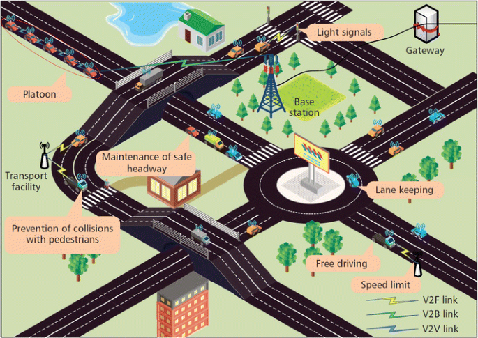
Descriptive text — Fig1: An image of the brain with continuous neural firings

Conventional deep learning models have achieved remarkable success in tasks such as image classification, language translation, and speech recognition. However, their rigid architectures and reliance on large, static datasets often leave them ill-suited for scenarios where conditions fluctuate rapidly or data is scarce. For instance, robotic agents operating in uncertain environments need to learn and adapt on-the-fly ^[1]. Similarly, autonomous vehicles must dynamically respond to variations in traffic patterns, weather conditions, or road anomalies. Liquid neural networks provide a mechanism for continuous adaptation, allowing these systems to not only perform well in dynamic contexts but also to generalize effectively beyond their training conditions ^[2] .

A visualization of dynamical contexts — Fig 2: Visualization of dynamical contexts which can be addressed by a Liquid Neural Network

Research into liquid neural networks is still in its early stages, yet the initial results are promising. By merging ideas from computational neuroscience, dynamical systems theory, and machine learning, liquid neural networks hold the potential to push the boundaries of what artificial systems can achieve.

"We are thrilled by the immense potential of liquid neural networks, as it lays the groundwork for solving problems that arise when training in one environment and deploying in a completely distinct environment without additional training. These flexible algorithms could one day aid in decision-making based on data streams that change over time, such as medical diagnosis and autonomous driving applications" - Daniela Rus, CSAIL director and the Andrew (1956) and Erna Viterbi Professor of Electrical Engineering and Computer Science at MIT.

Background

The conceptual roots of liquid neural networks can be traced back to a lineage of research focused on bridging continuous-time dynamical systems with artificial intelligence. Well before the term “liquid neural networks” entered the lexicon, computational neuroscientists and machine learning researchers were investigating biologically inspired models that adapt their internal parameters in real time. Early groundwork came from the study of continuous-time recurrent neural networks (CTRNNs) ^[3], which used differential equations to capture the evolving state of neurons over time, and liquid state machines (LSMs) ^[4], which employed biologically plausible spiking units and reservoir computing principles to process time-varying inputs. These foundational ideas provided the fertile conceptual soil from which the notion of liquid neural networks would emerge.

In the years leading up to the formal introduction of liquid neural networks, there was a growing recognition that conventional artificial neural architectures—often reliant on discretized time steps and fixed parameters—could not fully replicate the flexibility and adaptability observed in natural brains. Researchers at MIT CSAIL and other institutions began to probe this limitation more deeply, asking: Could we design networks that inherently adjust their dynamics as conditions change? This question set the stage for the eventual invention of liquid time-constant networks, a primary instance of liquid neural networks.

The key breakthrough came from a team led by Daniela Rus, Director of MIT CSAIL, and first author Ramin Hasani. Drawing upon their interdisciplinary backgrounds in robotics, dynamical systems, and computational neuroscience, the team devised a framework that introduced parameters governing neural dynamics as functions that continuously vary in time. They called these Liquid Time-Constant Neural Networks (LTCs) ^[2].

LTCs consists of a novel architecture where neurons dynamically adjust their time-constants based on input and hidden states. This is inspired by the dynamics of non-spiking biological neurons, emphasizing adaptability and stability in learning systems.

Methods

Here is a deep dive into the inner workings of an LTC, which is unfortunately, sparsely / not well covered in research papers. I wanted to get into the depths of what LTCs actually consist of, and why have they been constructed the way they are. I then show you important insights into its workings, through some clever design of experiments and analysis.

Derivation of LTC Model

Let us begin with the basic dynamics of a neural system represented by the state variable \(x(t)\), which evolves over time as a function of input \(I(t)\), time \(t\), and parameters \(\theta\). The most general form of such a system is an ODE given by:

\[\frac{dx(t)}{dt} = f(x(t), I(t), t, \theta)\] (1)

However, this approach relies heavily on implicit nonlinearities in the neural network \(f\), which limits its ability to capture complex temporal patterns. To overcome this, LTC networks introduce dynamic time-constants that depend on the input \(I(t)\) and state \(x(t)\). This adjustment enables neurons to act as specialized dynamical systems for different input features, enhancing the system's expressivity.

1. Adding a Linear Decay Term

To ensure stability and bounded dynamics, a linear decay term proportional to the state \(x(t)\) is introduced. This modifies the equation to:

\[\frac{dx(t)}{dt} = -\frac{x(t)}{\tau} + f(x(t), I(t), t, \theta)\] (2)

Here:

\(-\frac{x(t)}{\tau}\): Linear decay term, where \(\tau\) is the time constant.
\(f(x(t), I(t), t, \theta)\): Nonlinear term capturing the influence of inputs and parameters.

2. Introducing a Modulating Nonlinearity

We further enhance the system by defining \(f(x(t), I(t), t, \theta)\) as a product of a nonlinear function \(g\) and a term representing the equilibrium level \(A - x(t)\):

\[f(x(t), I(t), t, \theta) = g(x(t), I(t), t, \theta) \cdot (A - x(t))\] (3)

Substituting this into the equation gives:

\[\frac{dx(t)}{dt} = -\frac{x(t)}{\tau} + g(x(t), I(t), t, \theta) \cdot (A - x(t))\] (4)

3. Expanding the Dynamics

We expand the second term to separate the influence of \(x(t)\):

\[\frac{dx(t)}{dt} = -\frac{x(t)}{\tau} - g(x(t), I(t), t, \theta) \cdot x(t) + g(x(t), I(t), t, \theta) \cdot A\] (5)

Combining terms involving \(x(t)\), we get:

\[\frac{dx(t)}{dt} = -\left[\frac{1}{\tau} + g(x(t), I(t), t, \theta)\right] \cdot x(t) + g(x(t), I(t), t, \theta) \cdot A\] (6)

4. Defining the Liquid Time Constant

The effective time constant \(\tau_{\text{sys}}\) is defined as:

\[\frac{1}{\tau_{\text{sys}}} = \frac{1}{\tau} + g(x(t), I(t), t, \theta)\] (7)

5. Final Dynamics

Hence, the final governing equation for the LTC Network is:

\[\frac{dx(t)}{dt} = -\frac{x(t)}{\tau_{\text{sys}}} + g(x(t), I(t), t, \theta) \cdot A\] (9)

The neural network \(f\) not only determines the derivative of the hidden state \(x(t)\), but also serves as an input-dependent varying time-constant \(\tau_{\text{sys}} = \frac{\tau}{1+\tau \cdot f(x(t), I(t), t, \theta)}\) for the learning system. The time constant characterizes the speed and coupling sensitivity of an ODE. This property enables single elements of the hidden state to identify specialized dynamical systems for input features arriving at each time-point. Hence, these models were given the name: liquid time-constant recurrent neural networks (LTCs). LTCs can be implemented by an arbitrary choice of ODE solvers.

This formulation ensures that the dynamics of LTC networks are not only stable but also bounded, a critical requirement for real-world time-series modeling where inputs may grow unbounded.

Trainable Parameters in LTC Implementation
#	Parameter	Definition	Role
1	gleak	Leak conductance for each neuron.	Controls how quickly the neuron’s state decays toward its resting potential.
2	vleak	Leak reversal potential (resting state) for each neuron.	Defines the baseline voltage to which the neuron decays in the absence of input.
3	cm	Membrane capacitance for each neuron.	Determines the neuron’s ability to store charge, affecting input integration.
4	sigma	Scaling factor for sigmoid gating between neurons.	Modulates the strength of synaptic activation based on neuron states.
5	mu	Offset for the sigmoid gating function.	Controls the sensitivity of neuron interactions to presynaptic signals.
6	w	Synaptic weights between neurons.	Defines the strength of recurrent connections.
7	erev	Synaptic reversal potential.	Sets the equilibrium potential that synaptic currents drive neurons toward.
8	sensory_sigma	Scaling factor for sigmoid gating of sensory inputs.	Modulates the sensitivity of neurons to external inputs.
9	sensory_mu	Offset for sigmoid gating of sensory inputs.	Shifts the input-response curve for sensory neurons.
10	sensory_w	Weights for sensory inputs to neurons.	Determines how much influence each input dimension has on the neurons.
11	sensory_erev	Reversal potential for sensory input synapses.	Sets the equilibrium potential for sensory-driven currents.
12	input_w	Linear scaling weights for sensory inputs.	Multiplies raw input values before applying additional transformations.
13	input_b	Bias for sensory input mapping.	Adds a constant offset to sensory inputs after scaling.
14	output_w	Linear scaling weights for output neurons.	Determines how neuron states are combined to produce the output.
15	output_b	Bias for output mapping.	Adds a constant offset to the output after scaling.

Parameter Categories

Intrinsic Properties:
- gleak: Leak conductance
- vleak: Leak reversal potential
- cm: Membrane capacitance
Recurrent Dynamics:
- w: Weight matrix of recurrent connections
- sigma: Activation standard deviation
- mu: Activation mean
- erev: Reversal potential for recurrent connections
Sensory Inputs:
- sensory_w: Weight matrix for sensory inputs
- sensory_sigma: Standard deviation of sensory activations
- sensory_mu: Mean of sensory activations
- sensory_erev: Reversal potential for sensory inputs
External Inputs:
- input_w: Weight matrix for external inputs
- input_b: Bias for external inputs
Output Mapping:
- output_w: Weight matrix for output mapping
- output_b: Bias for output mapping

Quantifiable Relationships Between Parameters

\[ I_{recurrent} = w \cdot (\sigma \cdot activation(\mu, V)) \] (a)

\[ I_{sensory} = sensory\_w \cdot (sensory\_\sigma \cdot activation(sensory\_\mu, V)) \] (b)

\[ I_{input} = input\_w \cdot Input + input\_b \] (c)

\[ Output = output\_w \cdot State + output\_b \] (d)

\[ \frac{dV}{dt} = \frac{gleak \cdot (vleak - V) + I_{recurrent} + I_{sensory} + I_{input}}{cm} \] (e)

Experiments and Results

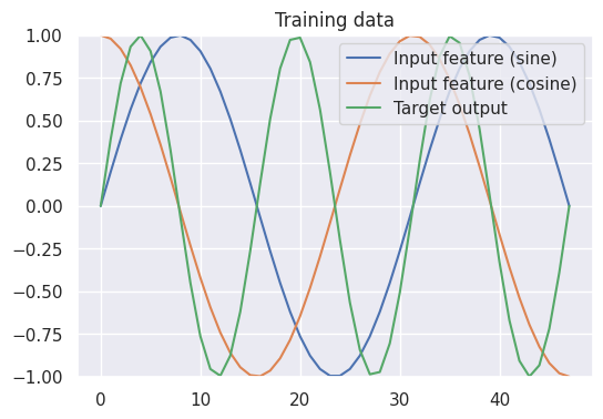
An experiment was designed to simulate time-series prediction task using synthetic data. The input feature consists of two signals: a sine wave and a cosine wave, both sampled over a length of \( N = 48 \). These input signals were generated using \( \sin \) and \( \cos \) functions over a range of \( 0 \) to \( 3\pi \). The target output is a sine wave with double the frequency of the input sine signal, generated over the same length. The input features were organized as a batch of size 1, resulting in a shape of \( (1, 48, 2) \), while the target output was reshaped to have a shape of \( (1, 48, 1) \). A visualization of the data reveals the relationship between the input signals and the target output, providing insight into the patterns the model is expected to learn.

Performance comparison across architectures — Fig 3: Training Data

For this experiment, the model employed a fully connected wiring scheme with 8 units, one of which was designated as a motor neuron to produce the output signal. This configuration was implemented using the FullyConnected wiring class. The model architecture consisted of two main layers: an input layer to accept sequences of two input features (sine and cosine waves) and the LTC layer with the defined wiring. The output of the LTC layer was configured to return sequences to match the time-series format of the target data.

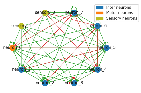
Neuron Types:

Motor Neuron (1): This neuron generates the output of the model, acting as the final layer. It connects to all other neurons to compute the output.
Interneurons (7): These neurons are recurrently connected and interact with each other. They capture temporal dependencies and dynamics within the LTC layer.
Sensory Neurons (2): These neurons handle the input data, connecting the input features (sine and cosine waves) to the interneurons.

The model was compiled using the Adam optimizer with a learning rate of 0.01 and a mean squared error loss function, which is suitable for regression tasks.

Analysis

1. Upon training the model, the recurrent weight matrix looks like:

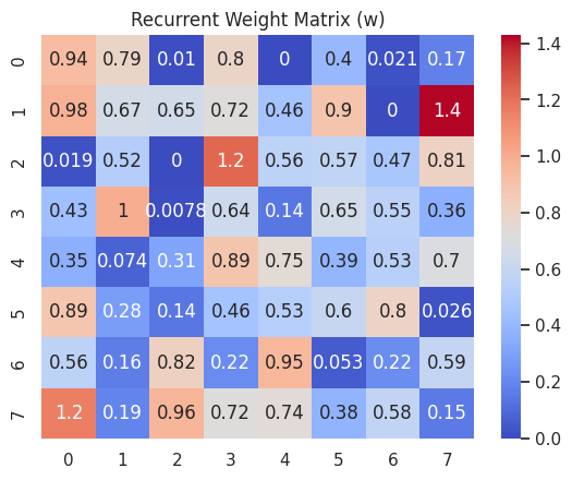
This represents the strength of connections between the neurons in the recurrent network. Each element w[i, j] in the matrix defines the weight of the connection from neuron j to neuron i.

Matrix Interpretation:

Rows correspond to the receiving neurons.
Columns correspond to the sending neurons.
The value of each element w[i, j]:
- Positive values indicate excitatory connections (enhancing the activity of the receiving neuron).
- Zero or near-zero values imply weak or no connection between the neurons.

This visualization highlights how the network neurons interact and provides insights into the model's temporal dynamics.

2. Next, we look at the impact of varying the leak conductance parameter (gleak) on the neuron dynamics in the LTC model. By adjusting gleak to different values (0.1, 0.5, and 1.0) and observing the model's predictions, the analysis highlights how this parameter influences the temporal behavior of the network.

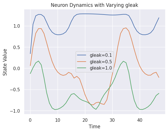
The results are visualized in a plot where the state values over time are compared for each gleak value. Lower gleak values result in slower decay or prolonged activity, while higher values lead to faster decay and reduced persistence of neuron states.

3. The next experiment explores the effect of perturbing sensory parameters in the LTC model on its output dynamics. Three key sensory parameters were modified:

sensory_w: The sensory weights, scaled by factor of 2.0.
sensory_mu: The sensory mean, shifted by adding 0.2.
sensory_sigma: The sensory standard deviation, broadened by a factor of 1.5.

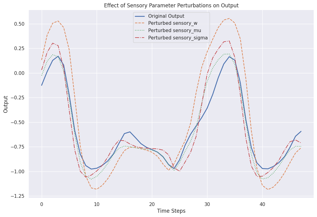
1. Scaling sensory_w (Sensory Weights):

These weights determine how strongly the input features influence the neurons. Scaling them affects the magnitude of the contribution from sensory inputs, thereby altering the overall network output. Smaller weights reduce the input's influence, while larger weights amplify it.

2. Shifting sensory_mu (Sensory Mean):

The mean (mu) represents the baseline or threshold for input activation. Shifting mu changes the input's bias, altering when and how the neurons respond to the inputs. For example, increasing mu requires larger input signals to achieve the same level of neuron activation, hence modifying the activation threshold.

3. Broadening sensory_sigma (Sensory Standard Deviation):

The standard deviation (sigma) controls the sensitivity to input variability. Broadening sigma (e.g., scaling by 1.5) increases the range over which inputs influence the neuron, potentially smoothing the response and making the network less sensitive to small changes in input.

These changes illustrate the interpretability and flexibility of the LTC model. The perturbations allow us to observe how specific parameter adjustments influence the temporal behavior and outputs of the network.

4. The next experiment conducts a global sensitivity analysis to evaluate the impact of perturbing individual trainable parameters in the LTC layer on the model's output. By applying small random perturbations to each parameter and measuring the resulting change in the model's predictions, the sensitivity of each parameter is quantified.

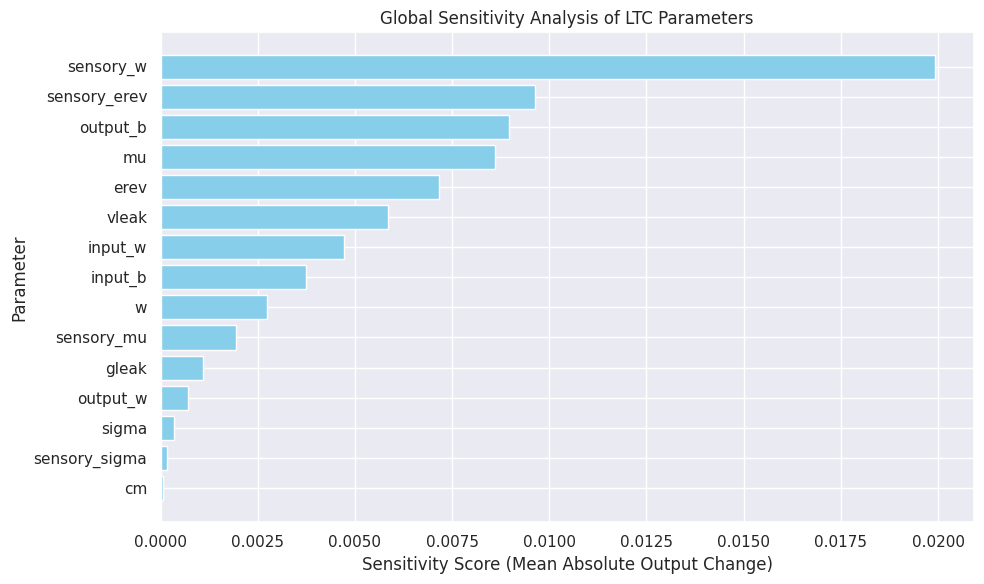
The sensitivity score for a parameter is computed as the mean absolute difference between the model's output with the perturbed parameter and the original output. This analysis provides insight into which parameters have the most significant influence on the model's behavior, helping to identify key components of the LTC dynamics.

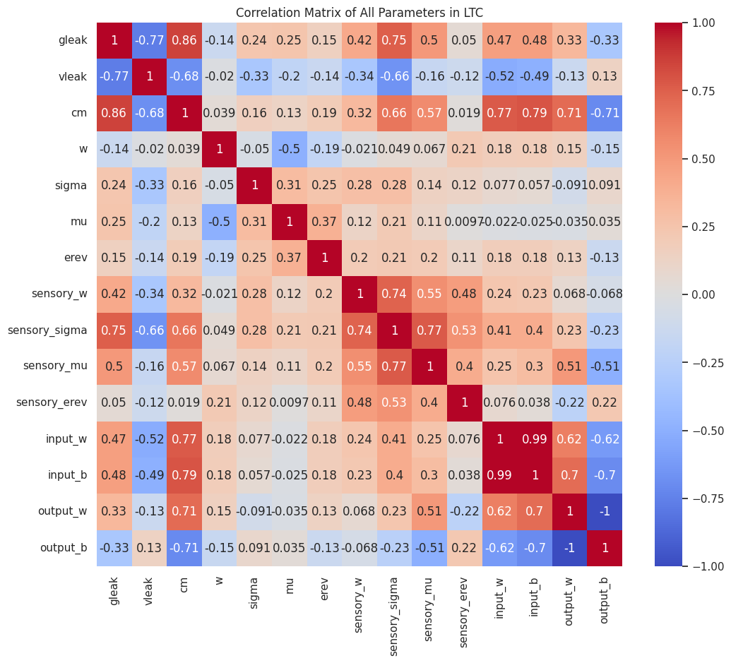
5. Finally, I explore the relationship between the trained parameters in the LTC layer by examining their pairwise correlations. The parameters include both neuron-specific values (e.g., gleak, vleak, cm) and connection-specific values (e.g., w, sigma, mu, and sensory parameters). Each parameter is extracted, flattened, and padded to ensure consistent lengths for correlation computation.

A correlation matrix is calculated to capture the degree of linear association between all pairs of parameters. This matrix provides insights into how changes in one parameter might relate to changes in another, highlighting dependencies or redundancies in the model's learned dynamics.

The correlation matrix is visualized as a heatmap, with parameter names labeled along the axes. Colors indicate the strength and direction of correlations:

Red tones represent strong positive correlations.
Blue tones indicate strong negative correlations.
White or neutral tones signify little to no correlation.

This visualization provides a clear and interpretable overview of parameter interactions within the LTC layer.

Discussion

The experiments conducted using the Liquid Time-Constant (LTC) model offer us valuable insights into its behavior, interpretability, and effectiveness in capturing temporal dynamics in a time-series prediction task. The use of synthetic data, combined with targeted parameter modifications, highlights the model's ability to adapt to complex temporal relationships and provides a framework for understanding its internal mechanisms.

Through the visualization of the recurrent weight matrix, we observe how the strength of connections between neurons facilitates the propagation of temporal information. The analysis of neuron dynamics with varying gleak values demonstrates how the leak conductance regulates signal decay, influencing the stability and responsiveness of the network. Moreover, the perturbation of sensory parameters (sensory_w, sensory_mu, sensory_sigma) reveals the flexibility of the LTC model in adjusting its sensitivity to input features. The ability to scale, shift, and broaden the influence of input signals underscores the adaptability of the model and its potential for handling diverse data patterns. These experiments validate the LTC's capability to integrate input signals in a controlled and interpretable manner.

The global sensitivity analysis further emphasizes the importance of individual parameters, identifying key contributors to the model's predictive behavior. This systematic evaluation helps prioritize parameters for fine-tuning and offers insights into the LTC's inner workings. Similarly, the exploration of parameter correlations provides a broader understanding of interdependencies within the model, revealing potential redundancies or synergies that could inform future model refinements.

Overall, the experiments demonstrate the LTC model's robustness and interpretability. The ability to analyze its parameters and their interactions enables a deeper understanding of its temporal dynamics, making it a powerful tool for time-series prediction tasks. These observations also align with the model's design to emulate biologically inspired dynamics. Future work could extend these findings to complex real-world datasets and explore more complex wiring configurations to further enhance the model's applicability.

Few other observations based on experiments I ran, but didn't include in the blog:

On simple synthetically derived datasets, vanilla RNNs do as well as LTCs, as there isn't much complexity. However, on more complex datasets, LTCs outperform RNNs. This is because LTCs can adapt their time-constants to the data, while RNNs cannot. This is a key property that makes them more powerful than vanilla RNNs. Some of the other important advantages of LTCs that I could conclude from my experiements and literature were:

Bounded Dynamics: Ensures the state \(x(t)\) remains finite.
Adaptivity: The time constant \(\tau_{\text{sys}}\) dynamically adjusts based on input and state.
Expressivity: The nonlinear modulation enables modeling of complex temporal patterns.

Limitations

While Liquid Time-Constant (LTC) models show significant promise in capturing temporal dynamics and performing well across various time-series prediction tasks, they also come with notable limitations that warrant further investigation:

1. Long-Term Dependencies: Like many other time-continuous models, LTCs face challenges in capturing long-term dependencies due to the vanishing gradient problem during gradient descent training. This issue, highlighted in studies by Pascanu et. al. (2013) ^[5], limits their applicability in tasks that require learning patterns over extended temporal sequences.

2. Choice of ODE Solver: The performance of LTCs is heavily influenced by the choice of numerical implementation methods for solving the underlying ordinary differential equations (ODEs). While advanced variable-step solvers enable strong performance, using simpler methods like the explicit Euler solver can significantly impact their efficiency and accuracy. This dependency on solver choice introduces variability in their effectiveness.

3. Time and Memory Complexity: LTCs, while highly expressive, incur substantial time and memory costs during training and inference. In comparison, Neural ODEs^[6]are faster but lack the expressive power of LTCs. The trade-off between computational complexity and model expressiveness highlights the need for further optimization of LTC architectures to make them more resource-efficient while retaining their powerful representational capabilities.

References

Chahine, Makram, et al. "Robust flight navigation out of distribution with liquid neural networks." Science Robotics 8.77 (2023): eadc8892. https://www.science.org/doi/full/10.1126/scirobotics.adc8892
Hasani, Ramin, et al. "Liquid time-constant networks." Proceedings of the AAAI Conference on Artificial Intelligence. Vol. 35. No. 9. 2021. https://ojs.aaai.org/index.php/AAAI/article/view/16936
Beer, R. D. (1995). “On the dynamics of small continuous-time recurrent neural networks.” Adaptive Behavior, 3(4), 469–505 https://doi.org/10.1177/105971239500300405
Maass, Wolfgang. "Liquid state machines: motivation, theory, and applications." Computability in context: computation and logic in the real world (2011): 275-296. https://www.worldscientific.com/doi/abs/10.1142/9781848162778_0008
Pascanu, R. "On the difficulty of training recurrent neural networks." arXiv preprint arXiv:1211.5063 (2013). https://proceedings.mlr.press/v28/pascanu13.html
Chen, Ricky TQ, et al. "Neural ordinary differential equations." Advances in neural information processing systems 31 (2018). https://arxiv.org/abs/1806.07366